Why molecular language models matter for property prediction
A familiar problem in property prediction is that you can have plenty of molecules but not many trustworthy labels for the property you actually care about—solubility in a specific solvent, metabolic stability in a given assay, or a process-relevant melting point. Traditional QSAR pipelines often depend on hand-built descriptors and careful feature engineering, and graph models can be strong but still behave like “from scratch” learners when labels are scarce or noisy.
Molecular language models change the starting point. They learn reusable chemical patterns from large, unlabeled corpora of molecular strings, then adapt to your specific endpoint with relatively little labeled data. In practice, that can improve data efficiency, robustness across related tasks, and transfer to new chemotypes—while also introducing real costs: pretraining is expensive, downstream performance can hinge on subtle data leakage, and confident-looking predictions can still be wrong outside the training chemistry.
What exactly is the “language” in a molecule?
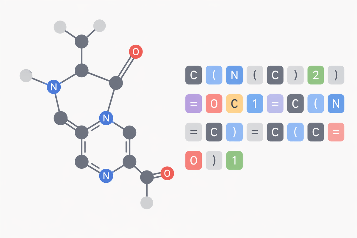
If you work with SMILES every day, the “language” idea sounds less mystical: it is simply a way to turn a molecule into a sequence of tokens that a text model can read. Characters like “C”, “N”, “=”, “( )”, and ring-closure digits encode connectivity, branching, aromaticity, and bond order. The model learns statistical regularities in these sequences—common substructures, typical local environments, and how certain patterns tend to co-occur—even before you show it a single property label.
The catch is that this language is not unique. The same molecule can have many valid SMILES depending on atom ordering, and small formatting choices (canonicalization, stereochemistry, salts) change the token stream. That can create avoidable variance, and sometimes “learning chemistry” collapses into “learning your writing conventions.” Many teams mitigate this with randomized SMILES augmentation or alternative tokenizations, but it is a practical cost: your preprocessing choices can matter as much as your model size.
Also, the sequence is a lossy interface to 3D reality. SMILES captures a 2D graph, while properties like permeability, conformational strain, and binding often depend on geometry and environment. Molecular LMs can still be useful here, but reliability depends on whether the property is largely determined by patterns that are visible in the string.
Pretraining objectives: what the model learns without labels
In pretraining, the model gets a game it can win using only unlabeled molecules: predict missing pieces of the sequence, or predict the next token given what came before. Masked-token objectives (BERT-style) force it to infer what “should” appear inside a local context—like reconstructing a ring closure digit, an aromatic pattern, or a typical heteroatom neighborhood. Autoregressive objectives (GPT-style) reward learning valid syntax and longer-range dependencies, such as how branches open and close or how certain motifs tend to follow others in real libraries.
Some setups add chemical structure signals without property labels: contrastive learning between different SMILES of the same molecule, or pairing a SMILES with a graph-derived view so the embedding stays stable across “spellings.” Others pretrain on reaction SMILES to learn transformations, which can help when endpoints correlate with synthesizability or scaffold evolution.
The “predict tokens well” is not the same as “predict solubility well.” Pretraining mostly teaches plausibility under the training distribution, so corpus bias and preprocessing choices can quietly shape what the model treats as normal chemistry.
From pretrained model to property predictor: the fine-tuning choices
A common moment after pretraining is realizing you still have to decide what “using the model” means: freeze it as a feature extractor, or update it end-to-end for your endpoint. Freezing is cheaper and more stable when you only have a few hundred labels; you embed each molecule once and train a lightweight head (often a small MLP) for regression or classification. Full fine-tuning can win when the endpoint is close to patterns the model already knows, but it is easier to overfit, especially if your labels come from a narrow project series.
Targets and losses matter more than teams expect. Many properties are noisy and assay-dependent, so robust losses, label transforms (e.g., log-scale), and careful handling of censored values can change rankings. Multi-task fine-tuning often helps when tasks share chemistry, but it can also dilute a high-value endpoint if the “auxiliary” tasks dominate the gradients. Class imbalance and scaffold splits force trade-offs: you can chase better random-split metrics, or accept lower scores that better reflect prospective risk.
Larger models increase GPU cost and hyperparameter sensitivity, and the best checkpoint on a validation set may still be miscalibrated for decision thresholds. If predictions will gate synthesis or screening, adding uncertainty estimates (ensembles, MC dropout, or conformal calibration) is usually worth the runtime overhead, because it turns “a number” into something you can triage and audit.
Where molecular LMs beat fingerprints or GNNs—and where they don’t
Teams often notice molecular LMs pulling ahead when labels are thin, endpoints are related to common medicinal-chemistry motifs, or you want one representation that can be reused across many assays. A pretrained LM can act like a strong default feature set: it tends to be less brittle than fixed fingerprints when scaffolds shift, and it can transfer across projects without rebuilding descriptors each time. It also handles “string-native” workflows well—deduping, augmenting with randomized SMILES, and batching large libraries for embeddings is usually straightforward.
Fingerprints still win on speed and simplicity. For many ADMET endpoints with plenty of historical labels, a well-tuned fingerprint + tree/linear model can be hard to beat per dollar, and it is easier to explain to stakeholders. Graph neural networks often outperform when the task depends on local topology and you have enough labels to learn it, especially if you can add 3D geometry or physicochemical features.
Molecular LMs struggle when the property is dominated by conformation, protonation state, solvent, or protein context that the SMILES does not encode. They also pay an operational tax: tokenization choices, longer training cycles, and failures that look “confident” unless you invest in calibration and applicability checks.
Data pitfalls that quietly break your benchmark
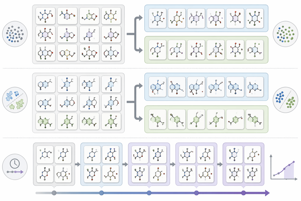
A benchmark can look “solved” because the train/test boundary is porous. The most common leak is near-duplicates: the same compound as different salts, tautomers, stereochemistry-stripped variants, or alternate SMILES that slip past a naive dedupe. Language models are especially good at exploiting this, because two spellings of the same scaffold can land very close in embedding space, inflating random-split scores without improving prospective hit rates.
Split choice is the second trap. Random splits mostly measure interpolation within a series; scaffold or time-based splits measure whether you can generalize to new chemistry or future batches. If your labels come from evolving assays, mixing old and new protocols in the same split can create a hidden “assay-ID” shortcut where the model learns conditions, not chemistry.
Finally, preprocessing decisions can quietly change the task. Standardizing protonation, stripping mixtures, or collapsing enantiomers may be necessary operationally, but it can also erase signal or mislabel pairs. Auditing these steps costs time, yet it is usually cheaper than chasing misleading leaderboard gains.
Making predictions usable: interpretability, constraints, and deployment
The typical usability test is a chemist asking “what should I change?” rather than “what score did it get?” Token-level attributions, substructure occlusion, or counterfactual SMILES edits can point to motifs driving a prediction, but they are only as meaningful as your representation: SMILES ordering artifacts and salt/protonation handling can produce explanations that track formatting. A pragmatic approach is to tie explanations back to standardized fragments (Murcko scaffolds, matched molecular pairs) and check whether the highlighted changes agree with known SAR, not just model gradients.
Constraints matter because many endpoints live inside workflow rules. If predictions gate synthesis, you usually need hard filters (reactivity flags, PAINS, charge ranges) alongside the model, because the LM will happily score molecules that violate your developability constraints unless it saw enough negatives. Uncertainty should be operational: calibrated intervals, “defer to experiment” thresholds, and an applicability-domain flag based on distance-to-training or conformal methods, even though ensembles and monitoring add runtime and engineering cost.
Deployment succeeds when the model is treated like a measurement device with drift. Version the preprocessing, freeze the label definition, log the input SMILES and standardization outputs, and track performance by chemical series over time. A slightly worse model with stable calibration, clear failure modes, and audit trails is often the one R&D teams will actually trust in prospective decisions.
A practical roadmap to choose your next experiment
A realistic starting point is to write down what you will do differently if the model is “right”: prioritize 50 compounds, kill a series, adjust a formulation screen. If that decision is cheap to reverse, try a frozen pretrained LM embedding plus a simple head and scaffold/time splits; you will learn quickly whether the signal is there without a large training bill. If the decision is expensive, require calibrated uncertainty and an applicability-domain flag before you look at point estimates.
Choose the representation to match the failure mode you can tolerate. If your endpoint is mostly 2D-structure driven and labels are scarce, an LM is often a good default. If 3D, solvent, or state dominates, budget for explicit physics/3D features or accept that the model is a triage tool, not a surrogate assay. Run one ablation you can explain to a project team: fingerprint baseline, LM embedding, and (if feasible) a GNN, all under the same split and standardization.
End with a prospective test that mirrors the workflow: a held-out time window, a new series, or the next batch. Log every preprocessing choice and treat “unknown” as a valid outcome. The goal is not the best retrospective score; it is a model that makes fewer costly mistakes per week of lab time.