Why simulate at all when you want to learn physics?
You usually simulate because the real system is slow, expensive, dangerous, or hard to instrument. If you’re trying to learn the dynamics of a drone, a factory robot, a fluid flow, or a battery pack, collecting enough high-quality trajectories in the real world can take weeks and still miss rare but important events. A simulator can generate millions of “what if” rollouts, label states you can’t easily measure, and let you rerun the same scenario to isolate causes.
The trade-off is that simulation gives you clean leverage at the price of potential wrongness. Every simplification—rigid bodies instead of flexible ones, ideal sensors, approximate friction, coarse meshes—can teach a model physics that only exists in the sim. Building and validating a simulator also costs real engineering time, and higher fidelity often means slower runs, which can erase the data advantage. Simulation helps most when you can bound the mismatch, or deliberately vary it so the learner stops relying on fragile details.
Done well, sim-trained learning is less about “replacing physics” and more about choosing where to spend certainty. You use known structure (conservation laws, constraints, priors) where it’s reliable, and you let learning fill in what’s unknown, unmodeled, or too complex to write down. The practical question isn’t whether simulation is realistic in an absolute sense; it’s whether it is realistic enough in the ways your downstream decisions depend on.
What counts as “the physical system” in your use case?
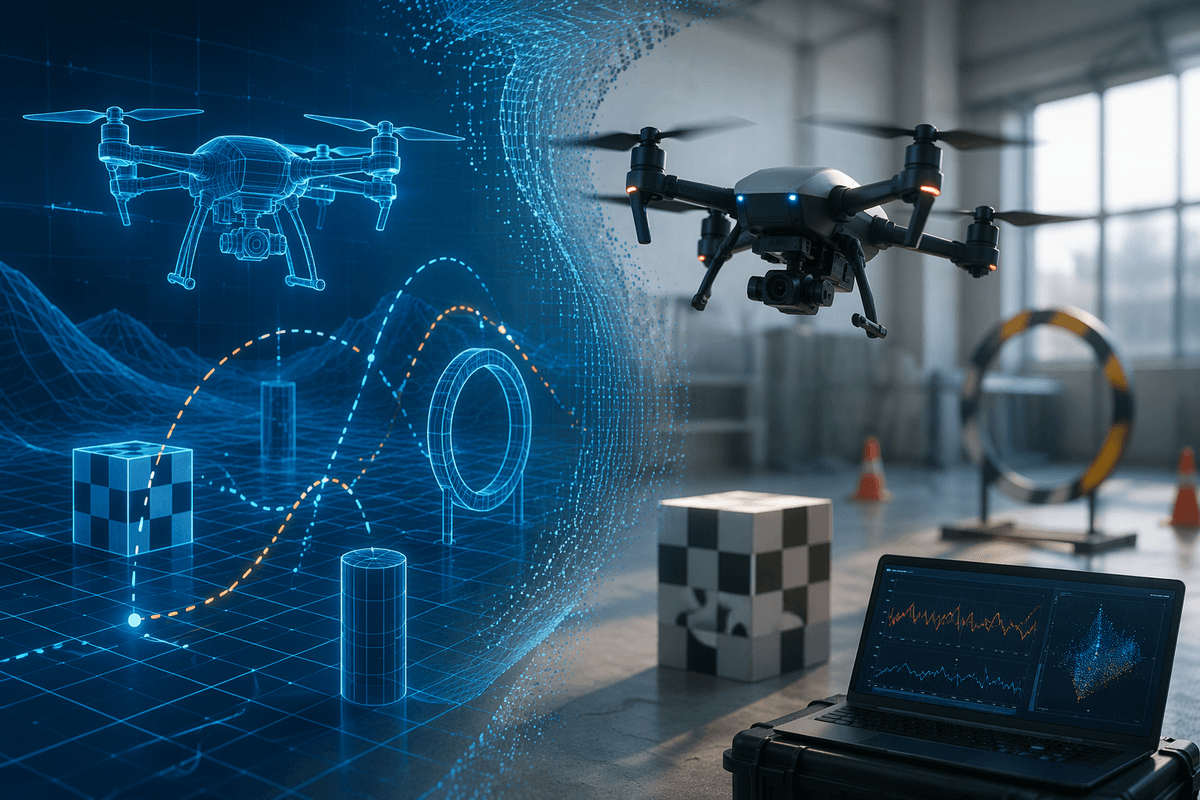
In practice, “the physical system” is whatever boundary makes your predictions stable and your decisions useful. A drone model that ignores wind might still work indoors, but outdoors wind is part of the system because it changes the mapping from motor commands to motion. The same applies to contact-rich robotics: if you treat friction as a fixed constant, but it varies with surface, temperature, or wear, you’re not modeling “the object” so much as a narrow lab setup.
The boundary usually has three layers: core dynamics (mass, geometry, constraints), interfaces (actuators, controllers, contacts), and observation (sensors, latency, filtering). Many sim-to-real failures are boundary mistakes: training on perfect state while deploying on noisy measurements; assuming instant actuation when real motors have lag; omitting cables, compliance, or backlash. Expanding the system costs you: more parameters to identify, more randomness to cover, and slower simulation. The workable choice is the smallest boundary that still captures the main failure modes you can’t tolerate.
Choosing a simulator: fidelity, speed, and controllable randomness
The simulator choice usually starts with an uncomfortable observation: the “best” simulator is often the one you can run enough times to cover your uncertainty. A high-fidelity CFD model might capture the right vortices, but if it takes hours per rollout, you’ll train on a narrow slice of conditions and overfit to them anyway. For many learning setups, a faster rigid-body or reduced-order model that runs 10,000× more episodes can beat a more accurate model simply by exposing the learner to more variation.
Fidelity matters most where errors change the decision. If you’re learning landing control, ground contact and actuator lag can dominate; mesh refinement in distant airflow may not. If you’re learning material deformation, “rigid body plus friction” is the wrong class of simulator no matter how much data you generate.
Controllable randomness is the lever that makes imperfect sims useful: randomize friction, mass, delays, sensor noise, and lighting within plausible ranges, then check that policies or predictors stay stable. The practical cost is engineering time: tuning randomization ranges, debugging nonphysical edge cases, and paying for compute when you scale rollouts.
Generating training data without teaching the wrong physics
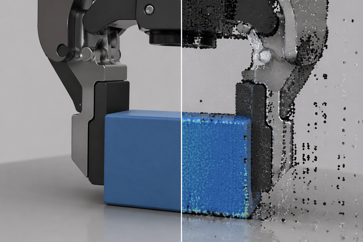
You can generate huge datasets in simulation and still end up with a model that fails on day one if the data mostly teaches simulator quirks. The common failure mode is “shortcut learning”: the predictor relies on artifacts like perfectly rigid contact, noiseless state, or a friction law that never changes. One practical guardrail is to start from the decisions you need to support (stability, safety margins, energy use) and ensure the dataset spans the regimes that stress them: slips, impacts, saturation, delays, and off-nominal initial conditions.
Diversity beats volume when you don’t know the true parameters. Domain randomization helps, but only if the ranges are defensible; too narrow and you overfit, too wide and you train on nonphysical worlds that dilute useful signal. It also helps to inject realistic observation and actuation imperfections during data generation—noise, dropout, quantization, latency—so the learner never sees a “privileged” state it won’t have at deployment. The cost is that debugging becomes harder, and training often needs more compute to converge.
Model options: black-box predictors vs physics-aware learners
A familiar fork shows up once you have trajectories: do you fit a flexible black-box predictor, or do you make the model “respect” physics on purpose? Black-box models (MLPs, CNNs, Transformers, diffusion-style forecasters) can learn fast and capture messy effects you didn’t encode. They also tend to extrapolate badly: push them into a new mass, a slightly different contact regime, or longer rollout horizons, and small one-step errors can compound into impossible states.
Physics-aware learners narrow the hypothesis space. You might parameterize known structure (rigid-body equations with learned friction), learn residual forces on top of a baseline simulator, or enforce constraints like conservation or non-penetration through the architecture or loss. The upside is often better sample efficiency and more stable rollouts under distribution shift. You must choose the right structure, implement differentiable pieces, and accept that the “wrong” physics prior can lock in systematic error that more data won’t fix.
In practice, hybrids win: a simple mechanistic core plus learned corrections, trained under the same noise and delays you expect at deployment.
Reality gap: how to know it will work outside simulation

A familiar warning sign is when a model looks stable in long simulation rollouts but becomes twitchy or biased the moment sensors, delays, and calibration drift show up. The reality gap is rarely one big missing effect; it’s usually many small mismatches that compound: contact is slightly softer, friction changes with humidity, a camera auto-exposure shifts, or a motor heats and loses torque. If your learned dynamics only ever saw “perfectly consistent” worlds, it will treat these shifts as surprises rather than normal variation.
The simplest test is not a headline metric, but a stress test: hold out entire regimes that look like deployment (new masses, surfaces, lighting, payloads), and check whether errors stay bounded over the time horizon your controller needs. Then do targeted real-world calibration on a small dataset: fit a few simulator parameters, or learn a residual correction, and see whether the correction is small and stable. If it needs large, brittle fixes, the sim is teaching the wrong causal story, and scaling rollouts won’t rescue it.
From prediction to control: using learned dynamics in decisions
A learned dynamics model becomes valuable when it sits inside a decision loop, not just a forecasting benchmark. In model-predictive control (MPC), you roll the model forward under candidate action sequences, score the outcomes (track a path, minimize energy, avoid collisions), then apply the first action and replan from the next measurement. That constant replanning is the practical hedge against model error: you only need the model to be locally reliable over the controller’s planning horizon, not perfect for minutes-long rollouts.
If the model is slightly optimistic about friction, the optimizer will choose aggressive maneuvers that “work” in simulation and fail on hardware. Guardrails usually mean adding conservative constraints, uncertainty penalties, or an ensemble that flags disagreement and forces safer actions. These choices have costs: more compute per decision, slower reaction time, and the need to tune safety margins so you don’t end up with a controller that is technically robust but too timid to be useful.
A practical checklist for starting your first sim-trained system
You can usually get traction by treating the first version as a credibility test, not a product. Write down the decision you need to make (track, grasp, stabilize, forecast) and the horizon it must work over, then list the few failure modes you cannot tolerate (slip, saturation, collision, thermal limits). Build the smallest simulator that reproduces those modes, and make the “deployment boundary” explicit: sensors, latency, actuation limits, and any upstream controller logic.
Randomize only what you can defend, and log it. Start with a short list (mass, friction, delays, noise) and widen ranges when real tests show bias, not because “more domain randomization” sounds safer. Hold out entire regimes as a reality-gap check, and budget time for parameter calibration or a learned residual on a small real dataset. Plan for the practical costs: rollout compute, debugging nonphysical edge cases, and extra inference time if you need ensembles or MPC to stay conservative.