Why sound source location is harder than it first seems
A common expectation is that locating a sound should be as simple as “which mic is louder.” That breaks quickly because real rooms add reflections that arrive milliseconds later and can be stronger than the direct path, especially near walls and tables. Two different positions can produce similar patterns across microphones, so the mapping from audio to location is not one-to-one.
Movement complicates it further. The source, the listener, and even the background can change while the sound is still unfolding, so the “where” depends on a time window choice. Then there’s microphone geometry: small spacing improves portability but reduces timing resolution; wider spacing helps, but makes devices bulkier and more sensitive to calibration drift. All of these constraints show up before you train a single model.
Define the task: Do you need angle, distance, or full 3D?
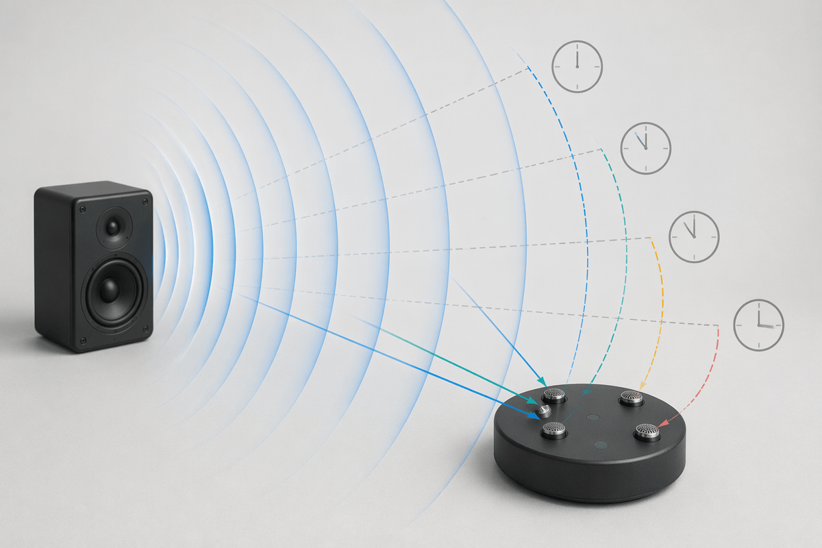
Most projects don’t need “a coordinate in space” so much as a decision that a product can act on. If you’re steering a camera, turning a robot, or lighting the right beamformer, angle-of-arrival (a direction) is often enough. That choice also matches what small microphone arrays can reliably provide, because timing differences mainly constrain direction, not absolute range.
Estimating distance is a different task. Loudness is unreliable across speakers and content, and reverberation can erase the simple relationship between amplitude and range. Some systems use multi-modal cues (audio plus vision), known emitted signals, or models that learn room-specific patterns, but the accuracy tends to collapse when the room or microphone placement changes.
Full 3D (azimuth, elevation, distance) raises the bar again: you need geometry that resolves elevation, careful synchronization, and labels that match the coordinate frame you’ll deploy in. Defining the output early prevents you from collecting expensive data for a target you can’t measure consistently.
Microphone setups that make learning feasible (and affordable)
A familiar failure mode is training on audio that “works” in headphones but collapses on a real device because the mic layout quietly changed. For learning-based localization, start with geometry you can reproduce: a 2‑mic pair for left/right direction on a small device, or a 4‑mic square (or linear bar) when you need stable azimuth across more angles. Arrays with spacings around a few centimeters are common because they fit hardware constraints while still producing measurable time differences at speech frequencies.
More microphones help, but cost shows up in boring places: synchronized sampling, consistent gain, and calibration. USB mics from different manufacturers often drift in timing and level, which teaches a model device-specific quirks instead of acoustics. A single multi-channel audio interface with matched mics, or an off-the-shelf dev board with a known array, is usually the cheapest way to keep the data “learnable.”
If elevation matters, you’ll need a non-coplanar setup (stacked layers or a 3D frame). That adds bulk and makes placement sensitivity worse, so it’s rarely worth it unless the product truly needs vertical separation.
Data you actually need: labels, rooms, noise, and motion
Once the array is fixed, the hard question becomes what “ground truth” you can label without lying to yourself. For angle-only systems, a clean label is often azimuth (and maybe elevation) relative to the array’s forward direction, which you can capture with a turntable, marked floor angles, or a motion-capture rig. For 3D position, you need coordinates in the same frame as the microphones, and small alignment errors (a few centimeters of mic position, a few degrees of rotation) can dominate your model’s apparent accuracy.
Room coverage matters as much as label quality. Data from one conference room teaches the model that room’s reflections; it may fail in a carpeted office or a kitchen. Collect across multiple rooms, multiple placements of the same array, and multiple source heights. If you can’t, simulate impulse responses to widen conditions, but expect a gap when you deploy because simulations rarely match messy surfaces and furniture.
Noise and motion decide whether it works outside demos. Mix in HVAC hum, keyboard clicks, and other talkers, and record with the source moving and the device rotating, not just static tripod takes. The cost is time: labeling moving sources is expensive, and multi-speaker scenes can turn “where is it?” into “which one do you mean?” unless your dataset defines that clearly.
Model approaches: from classic TDOA features to deep end-to-end
If you’ve ever clapped and noticed the sound “pull” toward a wall, you’ve already met the core modeling problem: you want the direct-path timing, but the microphones capture a mix of direct and reflected arrivals. Classic approaches start by estimating time-difference-of-arrival (TDOA) between mic pairs, often via cross-correlation (commonly GCC-PHAT), then fitting a direction that best explains those delays given your array geometry. This pipeline is interpretable and cheap to run, but it degrades when speech is intermittent, the room is highly reverberant, or there are multiple active sources.
A step up is a probabilistic tracker on top: treat each frame’s direction as noisy, then smooth it over time with a Kalman/particle filter. That helps products because it reduces jitter, but it adds knobs (process noise, update rate) that need tuning per device and motion pattern.
Deep learning typically replaces hand-built TDOA features with inputs like multi-channel STFT phase/complex spectra and outputs a direction class (angle bins) or regression vector. It can learn reflection-robust cues, but it’s data-hungry and can memorize room and device quirks, so training and deployment hardware must match more closely than teams expect.
Training choices that decide whether it generalizes or overfits
A familiar trap is getting “great accuracy” by splitting your dataset randomly, then discovering the model mostly learned a room signature. The safer split is by room and by physical setup: hold out entire rooms, microphone placements, and even a different unit of the same hardware if you have it. If performance drops sharply, that’s not a failure of the split; it’s a warning that your training data is too narrow for your deployment plan.
Augmentation is usually the cheapest way to buy robustness, but it has to match reality. Add noise at varied SNRs, convolve with diverse impulse responses, and randomize small timing and gain mismatches between channels to mimic calibration drift. Also vary source distance and height even if you only predict angle, because those changes reshape reflections. Collecting or curating impulse responses and verifying augmentations don’t break synchronization can take longer than model tuning.
Output design affects overfitting more than people expect. Angle classification into bins often trains more stably than pure regression, and you can smooth targets (soft labels) to reduce “edge” errors. Track a calibration-free metric (like median angular error) on held-out rooms, and stop training when that stops improving, even if training loss keeps falling.
Evaluation and deployment: what breaks first in the real world
The first thing that breaks in deployment is usually not the network, but the assumptions behind your eval. A model that looks stable on held-out clips can become jumpy when the device is handheld, when the speaker pauses mid-utterance, or when a second talker appears off-axis. Metrics should reflect that: report error over time (not just per-frame), measure how quickly it reacquires direction after silence, and include “unknown/ambiguous” cases rather than forcing a guess.
Hardware mismatch shows up fast. A few samples of channel skew, an automatic gain control you didn’t record with, or a different mic mesh can shift phase enough to move the predicted angle by tens of degrees. Budget time for a device-level validation pass: record a small, repeatable sweep around the array for every hardware revision, and track drift across temperature and battery states.
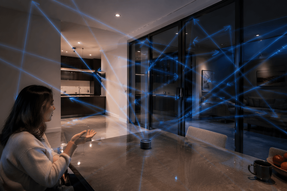
Room edges are the other cliff. Doorways, kitchens, and glass walls create reflection patterns your dataset likely under-sampled, so test in those “annoying” spaces on purpose. If compute is tight, expect to trade model size for latency; a slightly worse angle estimate that updates fast can outperform a better model that lags and overshoots.
Putting it together: a pragmatic roadmap for your first system
The most reliable first build is angle-only, indoors, with a fixed array you can reproduce. Start with a 4‑mic square or bar on a single multi-channel interface, record a simple azimuth sweep in three very different rooms, and lock a split that holds out rooms and device placements. Implement GCC-PHAT + geometric fitting as a baseline before training anything; if it fails badly, your labels, synchronization, or SNR assumptions are probably wrong.
Then add a small classifier on multi-channel STFT features, trained with impulse-response convolution, noise mixes, and randomized per-channel delay/gain jitter. Decide early what the product does when direction is uncertain (hold last, output “unknown,” or widen a beam), because real usage includes silence and competing talkers. Plan for a recurring “hardware sweep” test per revision; it costs time, but it prevents invisible mic changes from becoming model regressions.